Essays

So far we have seen that consumers exhibit behavior, called a demand curve, that differs from what they are physically capable of exhibiting called the spending curve. Simply put, consumers generally don't spend the same amount of money on any item or combination of items regardless of price. Instead, they tend to spend less money when prices rise because other items tend to attract their interest at that price, and they spend less money when prices decline because they become satiated with that item.

As a consequence of this behavior, there necessarily must be a particular combination of price and quantity at which point consumers are willing and able to spend the maximum amount of money. This "revenue maximum" we will call Rmax for short. The Rmax point occurs because there is only one possible point where the demand curve can touch the spending curve.

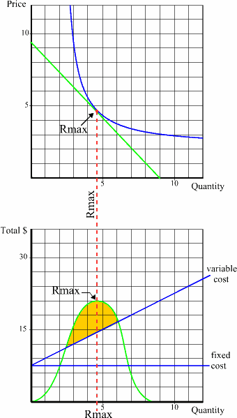
This means, in turn, that if we were to graph total revenues against quantity (using a graph with exactly the same quantity axis), we would find that total revenues (price times quantity) were low when the quantity sold was low but would rise rapidly as we began to sell quantities near the Rmax point. At precisely the Rmax point the total spending curve would become absolutely horizontal and then at quantities greater than the Rmax point the amount of total revenues would begin to decline until they became low again.

In other words, the somewhat bell shaped green curve on the lower graph corresponds to the total revenues that our demand curve would produce at every combination of prices and quantities that consumers are willing and able to transact. Since we observe that consumers do not spend the same amount of money regardless of price, the total spending curve represents what we observe consumers are actually willing and able to spend when prices vary. The Rmax point is therefore both the peak of this total revenue curve, and the point where the demand and spending curves touch. If our graph has the same quantity axis then these two points will both be on the dashed red vertical line.

From the sellers point of view, however, total revenues are somewhat irrelevant. Sellers have to contend with costs: they have to spend money in order to have the things they are selling, plus they have to spend money in order to have a place to sell and other related costs. There are fundamentally two constructively different classes of cost, fixed and variable, that have radically different consequences on the consumer and the seller.

Fixed costs are simply those costs that have no relation to the quantity sold: the seller has to pay the landlord the same building rent regardless of how many items consumers buy. Rent is a fixed cost. Insurance on the building and inventory is also the same regardless of how many items are sold. If you total up these fixed costs and plot them on a graph with quantity sold on the horizontal axis, you simply get a horizontal line above this axis because by definition the amount of fixed costs is the same at all quantity values.

Variable costs are simply those costs that depend on how many items you sell. If you sell paperback books at $5 each but buy them at wholesale for $3 each, then your total cost for buying books will depend on how many books you sold (assuming a constant inventory). If you sold a thousand books then your cost for books was $3,000 but if you sold two thousand books then your cost for books was $6,000 because each book you sell costs you more money. The same is true of paper bags: the more books you sell the more bags you give out to customers. Thus any plot of variable costs on a graph with quantity sold on the horizontal axis will be a line angling upward from zero at zero sold to some higher value at the end of the period.

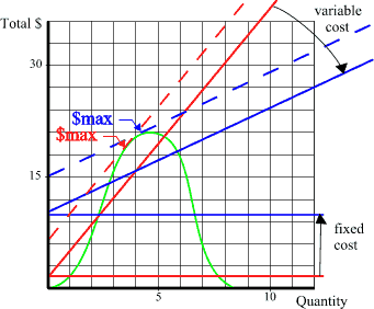
To figure out total costs you simply add fixed and variable costs together. To display this on a graph, you simply draw the (blue) horizontal fixed cost curve above the horizontal axis (meaning these costs have the same total no matter what the volume of sales) and then draw the (blue) variable cost line starting at the fixed cost line at zero quantity, sloping upward from there. The variable cost curve may not be actually straight: it may curve upward if costs tend to become greater at higher quantity volumes, or it may curve downward if there are "economies of scale" or other reasons costs might decline with volume (remember we are talking about total costs here, not per item costs where the fixed cost per item declines with volume). But a straight variable cost line is representative of costs over a short interval.

If you combine the (blue) total cost plot with the (green) total revenue plot, you will see that total revenue may actually be less than total costs at low quantities, then as total revenues rise they poke above total costs and reach the Rmax point before turning down again to fall below total costs again at high volumes. What this means is simply that total costs will invariably exceed total revenues at both high and low volumes with only a limited zone in between where total revenues exceed total costs.

Thus in between the two points where the total revenue and total cost curves cross, total revenues exceed total costs in that magical region where total profits exist: profits are the golden colored sector in the lower graph. Recognize, however, that at any given quantity of sales total profits are only the VERTICAL distance between the total cost curve and the total spending curve AT THAT QUANTITY, and therefore near the two crossing points the amount of profit is very small.

Consequently, once again we have a bell shaped curve to determine: total profits. If suppliers sell too few products, even at high prices, their overall profits will be small; if they sell more they will see greater profits until at some point more sales will result in lower total profits. There may very well be a broad range where suppliers can find some profits, but human nature (and market competition) will invariably push suppliers to search for the magical point of maximum profits.

Introduction | Previous | Next: The Point of Maximum Profits